# 常见函数的梯度

# 基础

• 导数 derivative
• 偏微分 partial derivative
• 梯度 gradient

$$\nabla f=\left(\frac{\partial f}{\partial x_1};\frac{\partial f}{\partial x_2};\ldots;\frac{\partial f}{\partial x_{n}}\right)$$

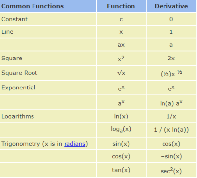
# 常见激活函数及其梯度

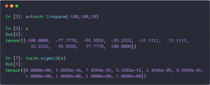
# Sigmoid / Logistic

$$f\left(x\right)=\sigma\left(x\right)=\frac{1}{1+e^{-x}}$$

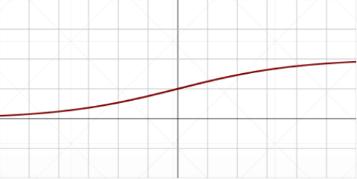
缺点，当 x 趋近于正无穷或负无穷时，$\sigma$ 趋近于 1 或 0，所以它的导数 $\sigma'$ 就会趋近于 0，造成梯度弥散

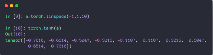
# Tanh

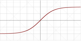
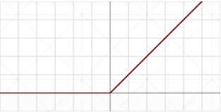
# ReLU

全称：Rectified Linear Unit

$$f\left(x\right)=\begin{cases}0 & \text{for }x<0\\ x & \text{for }x\ge0\end{cases}$$

$$f^{\prime}\left(x\right)=\begin{cases}0 & \text{for }x<0\\ 1 & \text{for }x\ge0\end{cases}$$

# 常见 Loss 及其梯度

# Mean Squared Error

注意 loss 和 L2 范式的区别如下

• loss = $\sum\left\lbrack y-\left(xw+b\right)^{}\right\rbrack^2$
• L2-norm = $\left\Vert y-\left(xw+b\right)\right\Vert_2$
• loss = $norm\left(y-\left(xw+b\right)\right)^2$

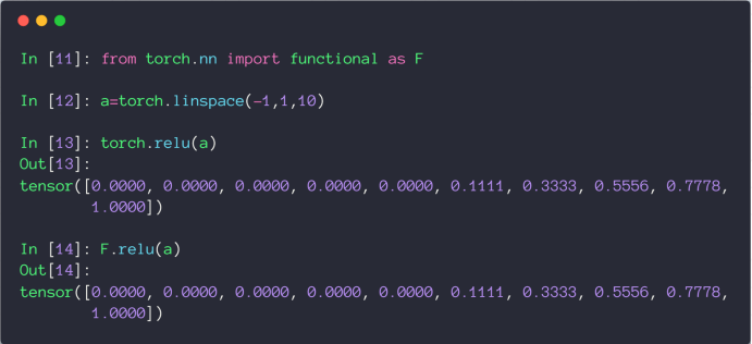
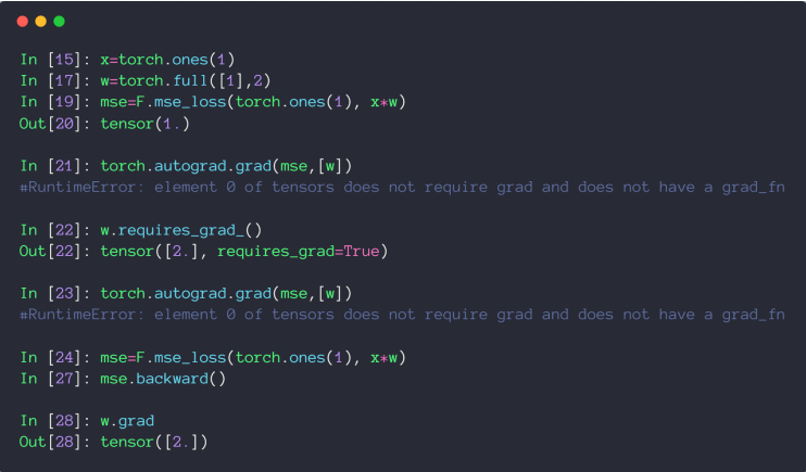
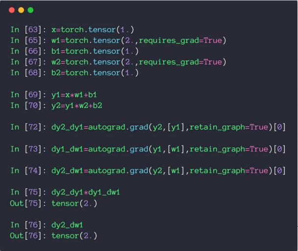
用 torch.autograd.grad 求参数的导数时，需要保证参数的 requires_grad 属性为 True，然后重新生成计算图

也可以用 backward 方法自动计算所有标记为可以求导的参数，赋值到参数的 grad 属性上

# Cross Entropy Loss

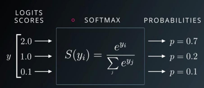
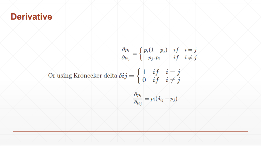
# Softmax 激活函数

和 Sigmoid 激活函数都可以返回 0-1 的近似概率值，但 Softmax 可以保证计算后的所有值的和为 1，同时会把大的值放的更大，小的值压缩到更小的空间～

# 代码案例

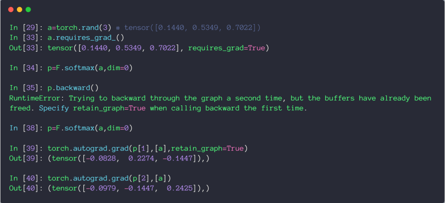
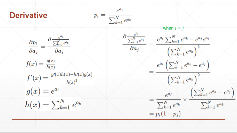
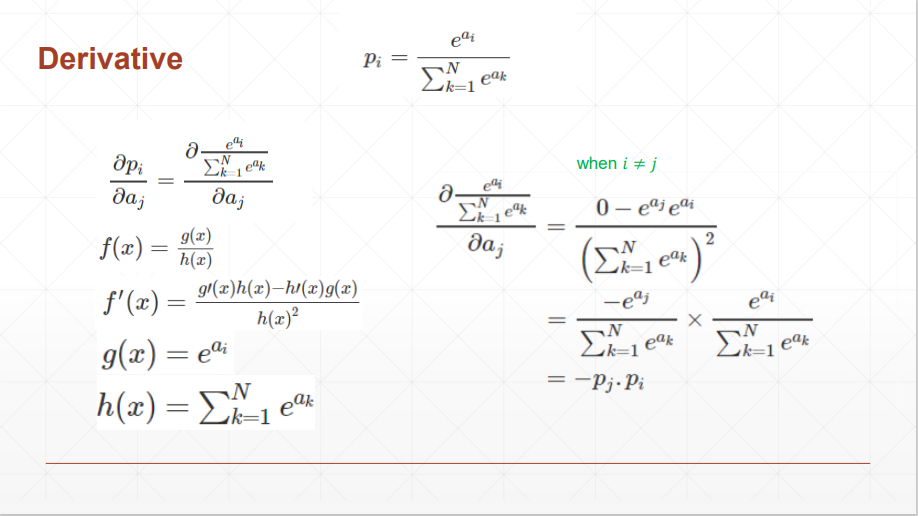
结论：当 i 和 j 相等时，导数为正，不等时，导数为负

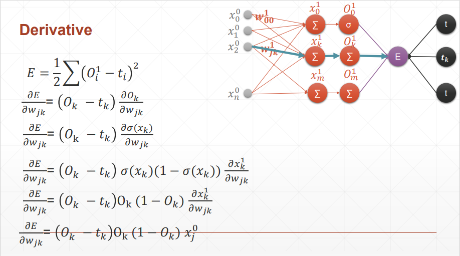
# 感知机的梯度推导

# 单层感知机

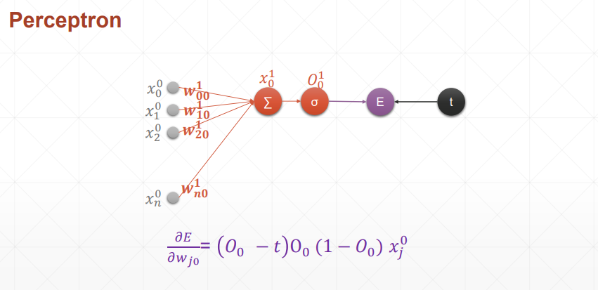
结论：损失函数对哪个参数求导，就和哪个参数有关，简洁美

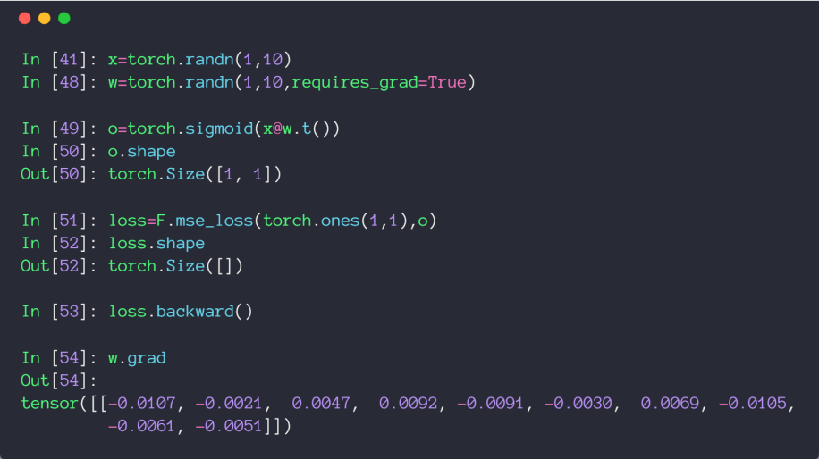
# 代码示例

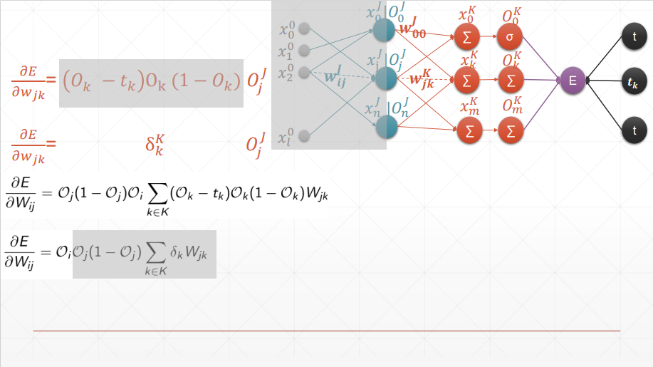
# 多层感知机

在梯度推导过程中，很巧妙的消掉了没有对 $W_{jk}$ 产生影响的部分，只有 $O_{k}-t_{k}$ 才会对 $W_{jk}$ 产生影响，所以求和符号就去掉了

结论：可以看到和单层感知机的区别就是 $O_0$ 变成了 O_

# 代码示例

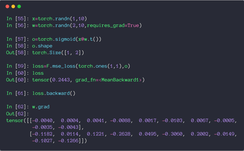
这里求损失函数时，应该写成 (1, 2)，为什么写成 (1, 1) 也不报错呢，因为符合 broadcasting，自动扩张了维度

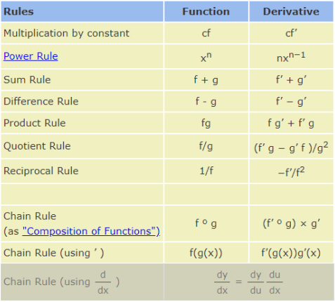
# 链式法则

# 基本规则

# 代码示例

可以验证链式法则结果的正确性

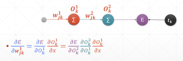
# 反向传播推导

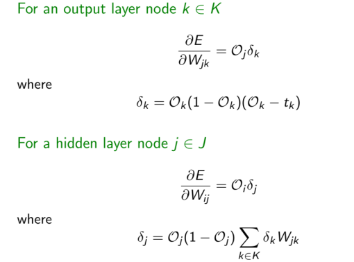
太优雅了，一环套一环的完成了反向传播

‍# 优化小实例

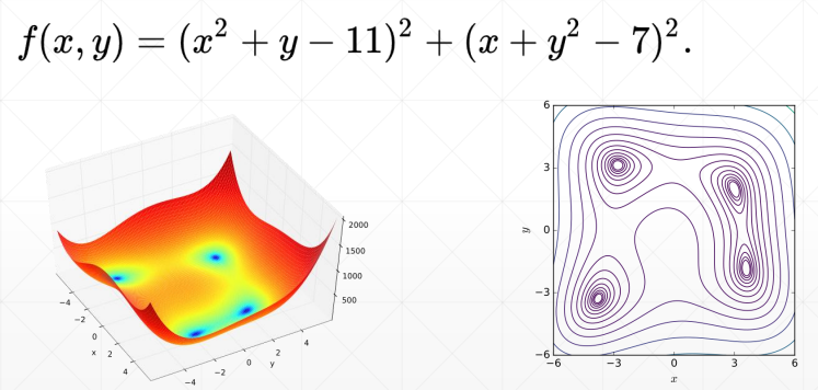
四个最小解

• f(3.0, 2.0) = 0.0
• f(-2.805118, 3.131312) = 0.0
• f(-3.779310, -3.283186) = 0.0
• f(3.584428, -1.848126) = 0.0

import  numpy as np

from    mpl_toolkits.mplot3d import Axes3D

from    matplotlib import pyplot as plt

import  torch

def himmelblau(x):

    return (x[0] ** 2 + x[1] - 11) ** 2 + (x[0] + x[1] ** 2 - 7) ** 2

x = np.arange(-6, 6, 0.1)

y = np.arange(-6, 6, 0.1)

print('x,y range:', x.shape, y.shape)

X, Y = np.meshgrid(x, y)

print('X,Y maps:', X.shape, Y.shape)

Z = himmelblau([X, Y])

fig = plt.figure('himmelblau')

ax = fig.add_subplot(projection = '3d')

ax.plot_surface(X, Y, Z)

ax.view_init(60, -30)

ax.set_xlabel('x')

ax.set_ylabel('y')

plt.show()

# [1., 0.], [-4, 0.], [4, 0.]

x = torch.tensor([-4., 0.], requires_grad=True)

optimizer = torch.optim.Adam([x], lr=1e-3)

for step in range(20000):

    pred = himmelblau(x)

    optimizer.zero_grad()

    pred.backward()

    optimizer.step()

    if step % 2000 == 0:

        print ('step {}: x = {}, f(x) = {}'

               .format(step, x.tolist(), pred.item()))